If f:R+→R+ is uniformly continuous with ∫a+∞f(t)dt<+∞, then t→+∞limf(t)=0.
For series we have n=1∑+∞un<+∞⇒n→+∞limun=0. However, for functions ∫a+∞f(t)dt<+∞⇎limt→+∞f(t)=0, the uniform continuity is necessary.
Example 1. f(x)=sin(x2)
Since ∫1+∞sin(x2)dxu=x2∫1+∞2usin(u)du, by Dirichlet’s test, the integral converges. However, x→+∞limsin(x2) does not exist.
Example 2. f(x)=1+x6sin2xx>0
Define F(u)=∫0uf(x)dx and ak=∫(k−1)πkπf(x)dx, then F(u) is monotonic increasing on R+ and F(nπ)=k=1∑nak. We have
ak≤∫(k−1)πkπ1+(k−1)6π6sin2xkπdx=2kπ∫02π1+(k−1)6π6sin2xdx≤2kπ∫02π1+(k−1)6π6(π2x)2dx=2kπ∫02π1+[2(k−1)3π2x]2dx=(k−1)3πk∫0(k−1)3π1+t2dt≤(k−1)3πk∫0+∞1+t2dt=2(k−1)3k+∞∼2k21
Here we use the inequality sinx≥π2x and the fact that ∫0+∞1+t2dt=2π. Therefore, n→+∞limF(nπ) exists. By F(x) increasing, x→+∞lim<+∞, but x→+∞limf(x) doesn’t exist.
Proof
If f(x)↛0 as x→+∞, then there exists ϵ>0 and a sequence (xn) such that ∀n∈N,∣f(xn)∣>ϵ. Since f is uniformly continuous, ∃δ>0∀n∈N∀y>0,∣xn−y∣<δ⇒∣f(xn)−f(y)∣<2ϵ. So ∀x∈[xn,xn+δ], we have ∣f(x)∣>∣f(xn)∣−∣f(xn)−f(y)∣>2ϵ. Therefore
However, since ∫0∞f(t)dt exists. LHS converges to 0 as n→+∞, yielding a contradiction. □
However, since ∫0∞f(t)dt exists. LHS converges to 0 as n→+∞, yielding a contradiction. □
which contradicts Gelfand’s formula. Therefore, Aα=α>0 which means there exists a positive eigenvector α with respect to eigenvalue ρ(A).
Assume that there exists an eigenvector β that is linearly independent with α and corresponds to the eigenvalue ρ(A)=1. Let c=minβi>0βiαi=βkαk (if β<0, we can choose −β>0), then we have c>0 and α−cβ≥0,α−cβ=0. However, since A>0, α−cβ=A(α−cβ)>0, which contradicts the fact that αk−cβk=0. Therefore, the geometric multiplicity of ρ(A) is 1.
Using the fact that AT is also positive, there exists a positive eigenvector γ with respect to the eigenvalue ρ(AT)=1. Note U=span(γ), we have Rn=U⊥⊕U. Since α>0,γ>0, then γTα>0⇒α∈U. Choose a basis E=(α,e1,⋯,en−1) for Rn, then the matrix of A under E is
(10∗B)
If there exists a positive eigenvector δ of B with respect to the eigenvalue 1, then δ∈UT, which implies δ and α are linearly dependent, contracting the fact that the geometric multiplicity is 1. Therefore, the algebraic multiplicity of A is also 1.
Suppose there exists a positive eigenvector β corresponding to the eigenvalue λ<1, then by the positivity of A, λ>0. Let c=maxβiαi=βkαk, then cβ−α≥0,cβ−α=0. However, since A>0, λcβ−α=A(cβ−α)>0, which means ∀i∈[[1,n]]λcβi>αi⇒c<λc<c, yielding a contradiction. Therefore, there are no other positive eigenvectors except positive multiples of α. □
If we use the dstribution Qθ(X) to approximate the distribution P(X), then
Minimizing forwad KL divergence θargminDKL(P∣∣Qθ) is equivalent to make a maximum likelihood estimation of θ under P.
Proof
θargminDKL(P∣∣Qθ)=θargminx∈X∑P(x)logP(x)−x∈X∑P(x)logQθ(x)=θargmaxEX∼P[logQθ(X)]+H(P) : Entropy of Px∈X∑−P(x)logP(x)=θargmaxEX∼P[logQθ(X)]=θargmaxi=1∏mQθ(xi)=θargmaxL(θ)=θMLE
Here we use Pdata={x1,⋯,xm} to represent the data we collected.
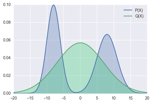
Wherever P(x) has high probability, Q(x) must also have high probability.
The figure above shows the effect of fitting a bimodal distribution P using a unimodal distribution Qθ through the forward KL divergence cost.
This property of the forward KL divergence is also often referred to as “zero avoiding”, because it tends to avoid having Q(x)=0 at any position where P(x)>0 .
Minimizing reverse KL divergence θargminDKL(Qθ∣∣P) is equivalent to requiring that the fitting maintains a single mode as much as possible.
Based on the properties of entropy, it is known that when Qθ approaches a uniform distribution, the value of H(Qθ(X)) is larger. Conversely, when Qθ tends toward a unimodal distribution (single-peak distribution), the value of H(Qθ(X)) is smaller. Therefore, the reverse KL divergence is equivalent to requiring Qθ to fit P while maintaining as much unimodality as possible.
Wherever Q(x) has high probability, P(x) must also have high probability.
The figure above shows the effect of fitting the same bimodal distribution P using a unimodal distribution Qθ through the reverse KL divergence cost.
The reverse KL divergence tends to minimize the difference between Qθ(x) and P(x) when Qθ(x)>0.
Let G be a finite group acting on a finite set X. For any x∈X, let Ox={g⋅x∣g∈G} be the orbit of x and Gx={g∈G∣g⋅x=x} be the stabilizer of x. Then
∣G∣=∣Ox∣⋅∣Gx∣
Proof
We construct a bijection between the orbit Ox and the set of left cosets of the stabilizer G/Gx. Define a map ϕ:G/Gx→Ox by ϕ(gGx)=g⋅x.
Well-defined: If g1Gx=g2Gx, then g2−1g1∈Gx, so g2−1g1⋅x=x⟹g1⋅x=g2⋅x. Thus ϕ is well-defined.
Injective: If ϕ(g1Gx)=ϕ(g2Gx), then g1⋅x=g2⋅x⟹g2−1g1⋅x=x⟹g2−1g1∈Gx, so g1Gx=g2Gx.
Surjective: For any y∈Ox, there exists g∈G such that y=g⋅x. Then ϕ(gGx)=y.
Since ϕ is a bijection, ∣Ox∣=[G:Gx]=∣Gx∣∣G∣. □
If G is a finite group and p is a prime number such that p∣∣G∣, then G contains an element of order p.
Proof
Consider the set S={(a1,…,ap)∈Gp∣a1…ap=e}. The first p−1 elements can be chosen arbitrarily, and ap is uniquely determined by ap=(a1…ap−1)−1. Thus ∣S∣=∣G∣p−1. Since p∣∣G∣, we have p∣∣S∣.
Let the cyclic group Zp=⟨σ⟩ act on S by cyclic shift: σ⋅(a1,…,ap)=(a2,…,ap,a1). Note that if a1…ap=e, then a1(a2…ap)=e⟹a2…ap=a1−1, so a2…apa1=a1−1a1=e. Thus the action is well-defined on S.
By the Orbit-Stabilizer Theorem, the size of any orbit divides ∣Zp∣=p. So the orbit sizes can only be 1 or p. Let k be the number of orbits of size 1. The elements in an orbit of size 1 satisfy a1=⋯=ap=a with ap=e.
Since S is the disjoint union of orbits, we have
∣S∣=k⋅1+m⋅p≡k(modp)
Since p∣∣S∣, we must have p∣k. Note that (e,…,e)∈S forms an orbit of size 1, so k≥1. Since p∣k, we must have k≥p≥2. Thus there exists at least one non-identity element a∈G such that ap=e. □
Every finite abelian group G is isomorphic to a direct sum of cyclic groups of prime power order. Moreover, the decomposition is unique up to reordering of the factors.
G≅Zp1e1⊕Zp2e2⊕⋯⊕Zpkek
where pi are primes (not necessarily distinct) and ei≥1.
Alternatively, it can be stated as:
Every finite abelian group G is isomorphic to a direct sum of cyclic groups of orders d1,d2,…,dk such that d1∣d2∣⋯∣dk>1.
G≅Zd1⊕Zd2⊕⋯⊕Zdk
The integers d1,…,dk are called the invariant factors of G.
Proof
The proof consists of two main steps: decomposing the group into its primary components (Sylow p-subgroups) and then decomposing each p-group into cyclic groups.
Step 1: Primary Decomposition
Let ∣G∣=n=p1e1p2e2…pkek be the prime factorization of the order of G.
For each prime factor pi, define the pi-primary component (or Sylow pi-subgroup) as:
G(pi)={x∈G∣∣x∣=pim for some m≥0}
Since G is abelian, G(pi) is a subgroup of G. We claim that G is the internal direct sum of these subgroups:
G≅G(p1)⊕G(p2)⊕⋯⊕G(pk)
Proof of decomposition:
Let mi=n/piei. Since gcd(m1,…,mk)=1, there exists integers u1,…,uk such that ∑i=1kuimi=1.
For any x∈G, we have x=x1=x∑uimi=∏i=1kxuimi.
Let xi=xuimi. Note that (xi)piei=xuimipiei=xuin=(xn)ui=eui=e. Thus ∣xi∣ divides piei, so xi∈G(pi).
So G=G(p1)…G(pk).
To show the sum is direct, suppose x1…xk=e with xi∈G(pi).
Fix j. Since ∣xi∣ is a power of pi, the order of y=∏i=jxi=xj−1 divides ∏i=j∣xi∣, which is coprime to pj.
But y=xj−1∈G(pj) has order a power of pj. The only element with order dividing two coprime numbers is the identity. Thus xj=e.
Thus, it suffices to prove the theorem for finite abelian p-groups.
Step 2: Structure of Finite Abelian p-groups
Let G be a finite abelian p-group. We proceed by induction on ∣G∣.
Let a∈G be an element of maximal order. Let H=⟨a⟩. We claim that H is a direct summand of G, i.e., there exists a subgroup K such that G=H⊕K.
Consider the quotient group G/H. By induction, G/H is a direct sum of cyclic groups. By lifting the generators of these cyclic groups back to G and adjusting them using the maximality of the order of a, one can construct the subgroup K.
Since ∣K∣<∣G∣, by the induction hypothesis, K is a direct sum of cyclic groups. Therefore, G=H⊕K is a direct sum of cyclic groups.
Combining these steps, any finite abelian group decomposes into a direct sum of cyclic p-groups. Grouping these appropriately yields the invariant factor decomposition. □