Probability Theory#

Markov / Chebyshev and Jensen’s Inequalities#

Markov’s Inequality

Let f be a non-negative measurable function and $t > 0$. Then, denote $\{f > t\} \vcentcolon= \{\omega \in \Omega : f(\omega) > t\}$,

$$\mu(\{f > t\}) \leq t^{-1} \displaystyle\int f \mathrm{d}\mu$$

Proof

Noting that $t\mathbf{1}_{\{f>t\}} \leq f$, then by monotonicity of the integral,

$$t\mu(\{f > t\}) = \displaystyle\int t\mathbf{1}_{\{f>t\}} \mathrm{d}\mu \leq \displaystyle\int f \mathrm{d}\mu$$

which proves the theorem.$\square$

There are two useful ways to use Markov’s inequality:

1. Chebyshev’s Inequality: For $f$ measurable and $m \in \mathbb{R}$, $$\mu(\{|f - m| > t\}) = \mu(\{(f - m)^2 > t^2\})\leq t^{-2} \displaystyle\int (f - m)^2 \mathrm{d}\mu \\ P(|X - \mathbb{E}[X]| > t) \leq \frac{\text{Var}(X)}{t^2}$$
2. Chernoff’s Inequality: For $f$ measurable and $m \in \mathbb{R}$, $$\mu(\{f > t\}) \leq e^{-tm} \displaystyle\int e^{mf} \mathrm{d}\mu \\$$ In probability theory, the right hand side becomes the moment generating function or the Laplace transform.

Convex Functions on $\mathbb{R}$

Let $I \subset \mathbb{R}$ be an interval. A function $\phi : I \rightarrow \mathbb{R}$ is convex if for all $t \in [0, 1]$ and all $x, y \in I$,

$$\phi(tx + (1 − t)y) \leq t\phi(x) + (1 − t)\phi(y)$$

Jensen’s Inequality

Let $(\Omega, \mathcal{F}, P)$ be a probability space and $X$ an integrable random variable ( i.e. a measurable function in $L^1(\Omega, \mathcal{F}, P)~$) such that $X : \Omega \rightarrow I \subset \mathbb{R}$. For any convex $\phi : I \rightarrow \mathbb{R}$,

$$\phi(\displaystyle\int X \mathrm{d}P) \leq \displaystyle\int \phi(X) \mathrm{d}P$$

which is $\phi(\mathbb{E}[X]) \leq \mathbb{E}[\phi(X)]$

Proof

For some $c \in I$, if $X = c$, $P$-a.e., then the result is immediate. Otherwise, let $m = \mathbb{E}[X]$ be the mean of $X$, which lies in the interior of interval. Then, we can choose $a, b \in \mathbb{R}$ such that $\phi(x) \geq ax + b$ for all $x \in I$ with equality at $x = m$. Then, $\phi(X) \geq aX + b$, and

$$\phi(\mathbb{E}[X]) = am + b = \mathbb{E}[aX + b] \leq \mathbb{E}[\phi(X)]$$

Lastly, to check that $\mathbb{E}[\phi(X)]$ is well defined (i.e. not $\infty−\infty$ ), we note that $\phi = \phi^+ −\phi^-$ where $\phi^-$ is concave and $\phi^-(x) \leq |a||x| + |b|$. Hence, $\mathbb{E}[\phi(X)] \leq |a|\mathbb{E}|x| + |b| < \infty$. $\square$

Hölder and Minkowski’s Inequalities#

Hölder’s Inequality

Let $p, q \in [1, \infty]$ be conjugate indices ( i.e. $\frac{1}{p} + \frac{1}{q} = 1$ ) and $f$ and $g$ be measurable, then $||fg||_1 \leq ||f||_p||g||_q$

Proof

If either $||f||_p = 0, \infty$ or $||g||_q = 0, \infty$, then the result is immediate. Hence, for $f$ such that $0 < ||f||_p < \infty$, we can normalize and without loss of generality assume that $||f||_p = 1$. Then, we can define a probability measure $P$ on $\mathcal{F}$ such that for any $A \in \mathcal{F}$,

$$P(A) \vcentcolon= \displaystyle\int_A f\mathrm{d}\mu$$

Then, using Jensen’s Inequality with $\phi(x) = x^q$ and $q(p − 1) = p$,

$$\begin{aligned} ||fg||_1 &= \displaystyle\int |fg| \mathrm{d}\mu = \displaystyle\int \frac{|g|}{|f|^{p - 1}}\mathbf{1}_{|f| > 0}\underbrace{|f|^p\mathrm{d}\mu}_{\color{#b984df}\text{prob measure }\mathrm{d}\nu} \\ &\leq \left[\displaystyle\int \left(\frac{|g|}{|f|^{p-1}}\mathbf{1}_{|f| > 0}\right)^q|f|^p\mathrm{d}\mu\right]^{\frac{1}{q}} \\ &\leq \left[\displaystyle\int |g|^q\mathrm{d}\mu\right]^\frac{1}{q} = ||f||_p||g||_q \end{aligned}$$

From Hölder’s inequality with $p=q=2$, we can derive Cauchy-Schwarz Inequality:

Cauchy-Schwarz Inequality

For measurable $f$ and $g$, $||fg||_1\leq||f||_2||g||_2$

Minkowski’s Inequality

Let $p \in [1, \infty]$ and $f$, $g$ be measurable functions, then $||f+g||_p\leq ||f||_p + ||g||_p$

Proof

If either $||f||_p = \infty$ or $||g||_p = \infty$ or $||f+g||_p=0$, then we are done. If $p=1$, then $|(f + g)(\omega)| \leq |f(\omega)| + |g(\omega)|$ and the result follows quickly. For $p\in (1, \infty]$ and $p, q$ conjugates, we note that

$$|||f+g|^{p-1}||_q = \left[\displaystyle\int |f+g|^{(p-1)q}\mathrm{d}\mu\right]^\frac{1}{q} = \left[\displaystyle\int|f+g|^p\mathrm{d}\mu\right]^{\frac{p-1}{p}} = ||f + g||^{p-1}_p$$

Then using the above equality, we have

$$\begin{aligned} ||f+g||^p_p &= \displaystyle\int |f+g|^p\mathrm{d}\mu \leq \displaystyle\int |f||f+g|^{p-1}\mathrm{d}\mu + \displaystyle\int |g||f+g|^{p-1}\mathrm{d}\mu \\ &\leq ||f||_p|||f+g|^{p-1}||_q + ||g||_p|||f+g|^{p-1}||_q \\ &= (||f||_p + ||g||_p)||f+g||^{p-1}_p \end{aligned}$$

Divide both sides by $||f + g||^{p−1}_p$ finishes the proof. $\square$

$L_p$ Approximation Theorem

Let $(\Omega, \mathcal{F}, \mu$) be a measure space, and let $\mathcal{A}$ be a $\pi$-system such that $\sigma(A) = \mathcal{F}$ and $\mu(A) < \infty$ for all $A ∈ \mathcal{A}$ and there exists $A_i \uparrow \Omega, A_i \in \mathcal{A}$. Let the collection of simple functions be

$$V_0 \vcentcolon= \left\{\displaystyle\sum_{i=1}^n a_i\mathbf{1}_{A_i} : a_i \in \mathbb{R}, A_i\in\mathcal{A}, n\in\mathbb{N}\right\}$$

For $p\in[1,\infty), V_0\subset L_p$ and for all $f\in L^p$ and all $\epsilon > 0$, there exists a $v\in V_0$ such that $||f-v||_p < \epsilon$.

Proof

For any $A \in \mathcal{A}, ||\mathbf{1}_A||_p = (\displaystyle\int\mathbf{1}_A\mathrm{d}\mu)^\frac{1}{p} = \mu(A)^\frac{1}{p} < \infty$. Thus $\mathbf{1}_A\in L^p$ for all $A\in\mathcal{A}$. Since $L^p$ is a linear space, $V_0 \subset L^p$.

Next, let $V\subseteq L^p$ be all $\mathcal{F}\in L^p$ that can be approximated as above by some $v\in V_0$ and $\epsilon > 0$. Let $f,g\in V$ be approximated by $v_f, v_g$ then by Minkowski’s Inequality,

$$||f+g - (v_f + v_g)||_p \leq ||f - v_f||_p + ||g - v_g||_p < 2\epsilon$$

Hence, $V$ is also a linear space.

Now, assume $\Omega\in\mathcal{A}$ ( i.e. $\mu(\Omega) < \infty$ ). Let $\mathcal{L} = \{B \in \Omega : \mathbf{1}_B\in V\}$, which we will show is, in fact, a $\lambda$-system. We know that $A \subset \mathcal{L}$ and thus $\Omega \in \mathcal{L}$. For $A, B \in\mathcal{L}$ such that $A\subseteq B$ then $\mathbf{1}_{B\setminus A} = \mathbf{1}_B - \mathbf{1}_A \in V$ since $V$ is linear, so $B\setminus A\in\mathcal{L}$. Lastly, for $\{A_i\}_{i=1}^\infty$ pairwise disjoint with $A_i \in \mathcal{L}$, let $A = \displaystyle\bigcup_{i=1}^\infty A_i$ and $B_j = \displaystyle\bigcup_{i=1}^j A_i$. Then, $B_j \uparrow A$ and $||\mathbf{1}_A − \mathbf{1}_{B_j}||_p = \mu(A \setminus B_j)^\frac{1}{p} \rightarrow 0$. Therefore, $A \in \mathcal{L}$, and thus $\mathcal{L}$ is a $\lambda$-system. By Dynkin $\pi$-$\lambda$ Theorem, $\mathcal{F}\subset\mathcal{L}$ and thus $\mathbf{1}_B\in V$ for any $B\in \mathcal{F}$. Therefore, for any non-negative $f\in L^p$, we can construct simple functions $f_n = \min\{n, 2^{-n}\lfloor 2^n\rfloor f\}$ such that $f_n\uparrow f$. Then $|f - f_n|^p\rightarrow 0$ pointwise and $|f - f_n|^p \leq |f|^p$. Hence, by Dominated Convergence Theorem, $||f - f_n||^p\rightarrow 0$. Thus $f \in V$ and by the linearity of $V$ , $V = L^p$.

Lastly, for general $\Omega$, we have by assumption a sequence $A_i \uparrow \Omega$. Hence, for any $f \in L^p$, we have that $f\mathbf{1}_{A_i} \in V$ and similarly to above, $|f − f\mathbf{1}_{A_i}|^p \rightarrow 0$ pointwise and $|f − f\mathbf{1}_{A_i}|^p \leq |f|^p$. Therefore, $||f − f\mathbf{1}_{A_i}||_p \rightarrow 0$ by dominiated convergence. Thus, $f \in V$. $\square$

Convergence of Measure#

Weak Convergence of Measure

Let $S$ be a metric space and $\mathcal{S}$ be the Borel $\sigma$-Field on $S$. Then, for a measure $P$ and a sequence $\{P_i\}_{i=1}^\infty$, we say that $P_i$ converges weakly to $P$, i.e. $P_i \Rightarrow P$, if

$$\displaystyle\int f \mathrm{d}P_i \rightarrow \displaystyle\int f \mathrm{d}P$$

for all $f\in \mathscr{C}^0_B(\mathbb{R})$, all continuous bounded real-valued functions on $S$.

Portmanteau Theorem

For $P$ and $P_i$ on a metric space $(S, \mathcal{S})$, the following are equivalent:

1. $P_i \Rightarrow P$
2. $\displaystyle\int f\mathrm{d}P_i\rightarrow\displaystyle\int f\mathrm{d}P$ for all bounded uniformly continuous functions $f$
3. $\displaystyle\limsup_i P_i(C) \leq P(C)$ for all closed sets $C$
4. $\displaystyle\liminf_i P_i(U) \geq P(U)$ for all open sets $U$
5. $\displaystyle\lim_i P_i(A) = P(A)$ for all sets $A\in\mathcal{S}$ with $P(\partial A) = 0$

Proof

• (1)$\rightarrow$(2) If convergence holds for every $f \in \mathscr{C}^0_B$ then is certainly hold for all bounded uniformly continous $f$.

• (2)$\rightarrow$(3) For any $C$ closed and $\epsilon > 0$ there exists a $\delta > 0$ such that for $C_δ = \{x \in S : d(x, C) < \delta\}$, we have $P(C_\delta) < P(C) + \epsilon$ as $C_\delta \downarrow C$ as $\delta\rightarrow 0^+$. Then, we can define an $f$ such that $f = 1$ on $C$, $f = 0$ on $S \setminus C_\delta$. Then $f$ is uniformly continuous (by Urysohn’s Lemma) and $0 \leq f \leq 1$ Then, by (2), we have that

  $$P_i(C) \leq \displaystyle\int f\mathrm{d}P_i\rightarrow\displaystyle\int f\mathrm{d}P \leq P(C_\delta) < P(C) + \epsilon$$

  Thus, taking the $\displaystyle\limsup$ and $\epsilon$ to zero gives $\displaystyle\limsup_i P_i(C) \leq P(C)$

• (3)$\rightarrow$(1) Let $f \in \mathscr{C}^0_B(\mathbb{R})$. Our goal is to show that $\displaystyle\limsup_i\displaystyle\int f \mathrm{d}P_i \leq\displaystyle\int f \mathrm{d}P$ and similarly for $\displaystyle\liminf$ to show (1) holds. As $f$ is bounded, we can shift and scale it, and without loss of generality, we assume that $0 < f < 1$. Then, for any choice of $n \in \mathbb{N}$, we define nested closed sets $C_j = \{x\in S : f(x)\geq j/n\}$ for all $j= 1, 2, \ldots, n$ and cut $f$ into pieces to get

  $$\displaystyle\sum_{j=1}^n\frac{j-1}{n}P(C_{j-1}\setminus C_j) \leq \displaystyle\int f\mathrm{d}P \leq \displaystyle\sum_{j=1}^n\frac{j}{n}P(C_{j-1}\setminus C_j)$$

  Also, $P(C_{j-1}\setminus C_j) = P(C_{j-1}) - P(C_j)$, the above becomes

  $$\frac{1}{n}\displaystyle\sum_{j=1}^n P(C_j) \leq \displaystyle\int f\mathrm{d}P \leq \frac{1}{n} + \frac{1}{n}\displaystyle\sum_{j=1}^n P(C_{j})$$

  Thus,

  $$\displaystyle\limsup_i \displaystyle\int f\mathrm{d}P_i \leq \frac{1}{n} + \frac{1}{n}\displaystyle\sum_{j=1}^n \displaystyle\limsup_i P_i(C_j) \leq \frac{1}{n} + \frac{1}{n}\displaystyle\sum_{j=1}^n P(C_j) \leq \frac{1}{n} + \displaystyle\int f\mathrm{d}P$$

  Taking $n \rightarrow \infty$ gives $\displaystyle\limsup_i \displaystyle\int f \mathrm{d}P_i \leq \displaystyle\int f \mathrm{d}P$. Replacing $f$ with $−f$ gives $\displaystyle\liminf_i f \mathrm{d}P_i \geq \displaystyle\int f \mathrm{d}P$. Thus the $\displaystyle\limsup$ and $\displaystyle\liminf$ coincide proving that (3)$\rightarrow$(1).

• (3)$\Leftrightarrow$(4) Let $U$ be the complement of $C$. Then, $P(U) = 1 - P(C)$ Thus, $\displaystyle\limsup_i P_i(C) \leq P(C)$ is equivalent to $\displaystyle\liminf_i P_i(U) \geq P(U)$.

• (3)(4)$\Leftrightarrow$(5) For any set $A\in\mathcal{S}$ with $P(\partial A) = 0$, $A^\circ$ is an open set and $\bar{A}$ is a closed set. If (3) and (4) hold, we have that

  $$P(A^\circ) \leq \displaystyle\liminf_i P_i(A^\circ) \leq \displaystyle\liminf_i P_i(A) \leq \displaystyle\limsup_i P_i(\bar{A}) \leq \displaystyle\limsup_i P_i(\bar{A}) \leq P(\bar{A})$$

  Since $P(\partial A)=0$, we have that $P(A^\circ) = P(\bar{A})$. This is equivalent to $\displaystyle\lim_i P_i(A) = P(A)$, which is (5). $\square$

Convergence of Random Variables#

In contrast to convergence of measures, let $(\Omega, \mathcal{F}, \mu)$ be a probability space and $(S, \mathcal{S})$ be a metric space with Borel sets as above. Then, for a random variable (i.e. measurable function) $X : \Omega → S$, we can define a probability measure

This is the distribution of $X$ . Then the expectation of a random variable can be written in multiple ways due to change of variables:

Note that above Portmanteau Theorem can be rephrased for random variables as well.

Convergence in Distribution

For a sequence of random variables $\{X_i\}_{i=1}^\infty$, we say that $X_i$ converges to $X$ in distribution ( denoted $X_i\overset{d}{\longrightarrow}X$ ) if $P_i \Rightarrow P$.

Convergence in Probability

For a sequence of random variables $\{X_i\}_{i=1}^\infty$, we say that $X_i$ converges to $X$ in probabilty ( denoted $X_i\overset{P}{\longrightarrow}X$ ) if for all $\epsilon > 0$

$$\mu(\{\omega \in \Omega : d(X_i(\omega), X(\omega)) > \epsilon\}) \rightarrow 0$$

In short, $P(d(X_i, X)>\epsilon)\rightarrow 0$.

This means that the measure of the set of $\omega$ where $X_i(\omega)$ and $X(\omega)$ differ by more than $\epsilon$ goes to zero as $i \rightarrow \infty$. Convergence in probability is closely connected to the metric $d$ on $(S, \mathcal{S})$.

Convergence Almost Surely

For a sequence of random variables $\{X_i\}_{i=1}^\infty$, we say that $X_i$ converges almost surely to $X$ ( denoted $X_i\overset{\text{a.s.}}{\longrightarrow}X$ ) if

$$\mu(\{\omega \in \Omega : X_i(\omega) \rightarrow X(\omega)\}) = 1$$

i.e. pointwise convergence almost everywhere.

Convergence in $L^p$

For a sequence of random variables $\{X_i\}_{i=1}^\infty$, we say that $X_i$ converges to $X$ in $L^p$ if

$$E[d(X_i - X)^p] = \displaystyle\int d(X_i(\omega), X(\omega))^p\mathrm{d}\mu(\omega) \rightarrow 0$$

Here, we can think of $d(X_i(\omega), X(\omega))$ as a function from $\Omega$ to $\mathbb{R}^+$. In the case that we have real valued random variables, i.e. $S = \mathbb{R}$, then this is

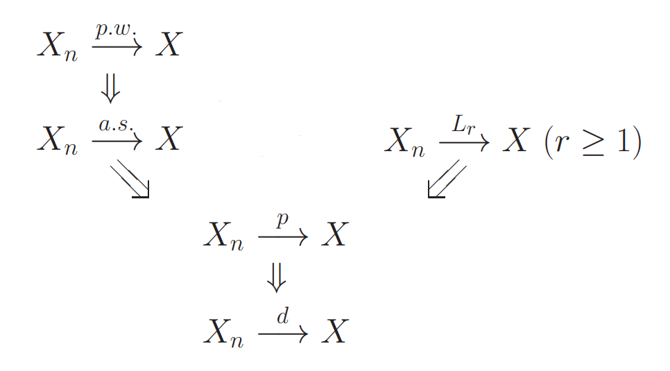
Hierarchy of Convergence Types#

• Conv a.s. $\Rightarrow$ conv in probability
• Conv in probability $\Rightarrow$ conv in distribution
• For $1\leq p < q \leq \infty$, conv in $L^q$ $\Rightarrow$ conv in $L^p$
• For any $p\in [1, \infty]$, conv in $L^p$ $\Rightarrow$ conv in probability

Borel-Cantelli Lemmas#

Let $(\Omega, \mathcal{F}, \mu)$ be a probability space. For $\{A_i\}_{i=1}^\infty, A_i\in \mathcal{F}$, then we define

The set $\displaystyle\limsup_i A_i$ is sometimes referred to as $A_i$ infinitely often or $A_i$ i.o. This is because $\omega \in \displaystyle\limsup_i A_i$ implies that for any $N \in \mathbb{N}$ there exists an $n > N$ such that $\omega\in A_n$. Similarly, some write $A_i$ eventually or $A_i$ ev. for $\displaystyle\liminf_i A_i$. This is because for $\omega \in \displaystyle\liminf_i A_i$ then there exists an $N$ large enough such that $\omega \in A_n$ for all $n \geq N$.

1st Borel-Cantelli Lemma

Let $\{A_i\}_{i=1}^\infty$ with $A_i \in \mathcal{F}$. If $\displaystyle\sum_{i=1}^\infty \mu(A_i) < \infty$, then $\mu(\displaystyle\limsup_i A_i) = 0$.

Proof

As the summation converges, then the tail sum has to tend to zero, we have simply that

$$\mu(\displaystyle\limsup_i A_i) = \mu\left(\displaystyle\bigcap_{i=1}^\infty\displaystyle\bigcup_{j > i} A_j\right) \leq \mu\left(\displaystyle\bigcup_{j > i} A_j\right) \leq \displaystyle\sum_{j > i} \mu(A_j) \rightarrow 0$$

as $i\rightarrow \infty$. $\square$

2nd Borel-Cantelli Lemma

Let $\{A_i\}_{i=1}^\infty$ be an independent collection with $A_i \in \mathcal{F}$. If $\displaystyle\sum_{i=1}^\infty \mu(A_i) = \infty$, then $\mu(\displaystyle\limsup_i A_i) = 1$.

Proof

Note that $1 − t \leq e^{−t}$ for all $t \in \mathbb{R}$ and we have that the independence of the $\{A_i\}_{i=1}^\infty$ implies the independence $\{A^c_i\}_{i=1}^\infty$. Therefore, for any $i \in \mathbb{N}$ and $k \geq i$,

$$\mu(\displaystyle\bigcap_{j=i}^k A^c_j) = \displaystyle\prod_{j=i}^k (1 - \mu(A_j)) \leq \exp\left(-\displaystyle\sum_{j=i}^k \mu(A_j)\right)$$

Taking $k \rightarrow \infty$ takes the right hand side to zero. Hence, $\mu(\displaystyle\cap_{j>i} A^c_j) = 0$ for all $i$. Thus,

$$\mu(\displaystyle\limsup_i A_i) = \mu\left(\displaystyle\bigcap_{i=1}^\infty\displaystyle\bigcup_{j > i} A_j\right) = 1 - \mu\left(\displaystyle\bigcup_{i=1}^\infty \displaystyle\bigcap _{j > i} A^c_j\right) = 1$$

which is the desired result. $\square$

Weak Law of Large Numbers#

Weak Law of Large Numbers

Let $(\Omega, \mathcal{F}, P)$ be a probability space and $\{X_i\}_{i=1}^\infty$ be random variables (measurable functions) from $\Omega$ to $\mathbb{R}$ such that $E[X_i] = c \in \mathbb{R}$ and $E[X_i^2]=1$ for all $i$ and $E[(X_i − c)(X_j − c)] = 0$ for all $i \neq j$. Then $\frac{S_n}{n} \overset{P}{\longrightarrow} c$.

Proof

Without loss of generality, we assume $c = 0$. Otherwise, we can replace $X_i$ with $X_i − c$. Then, for any $t > 0$, Chebyshev’s inequality implies that

$$P(\frac{|S_n|}{n} \geq t) \leq \frac{E[S_n^2]}{n^2t^2} = \frac{1}{n^2t^2}E[(\displaystyle\sum^n_{i=1} X_i)^2] = \frac{1}{n^2t^2}E[\displaystyle\sum^n_{i=1} X_i^2] = \frac{1}{nt^2} \to 0$$

as $n \to \infty$. $\square$

Note that in the above proof, we only require that the $X_i$ be uncorrelated (i.e. $E[(X_i −c)(X_j −c)] = 0$ ) and not independent. In the next theorem, we require independence, but remove all second moment conditions.

Strong Law of Large Numbers#

Strong Law of Large Numbers

Let $\{X_i\}_{i=1}^\infty$ be i.i.d. random variables from $\Omega$ to $\mathbb{R}$.

1. If $E[|X_i|] = \infty$, then $\frac{S_n}{n}$ does not converge to any finite value.
2. If $E[|X_i|] < \infty$, then $\frac{S_n}{n} \overset{a.s.}{\longrightarrow} c$ for $c = E[X_i]$.

Proof

1. Assume that $\frac{S_n}{n} \longrightarrow c \in \mathbb{R}$ but also that $E[|X_i|] = \infty$, and note that $\frac{X_n}{n} = \frac{S_n − S_{n−1}}{n} \to 0$. Since $E[|X_i|] = \infty$, then $\displaystyle\sum_{n=0}^\infty P(X_i > n) = \infty$ and 2nd Borel-Cantelli Lemma says that $|X_n| > n$ for infinitely many $n$. Thus

   $$P(\{\omega\in\Omega : \frac{S_n - S_{n-1}}{n}\to 0\}) = 0$$

   Thus $\frac{S_n}{n}\nrightarrow c \in \mathbb{R}$.

2. Assume that $E[X_i] = c \in \mathbb{R}$. Without loss of generality, we assume $X_i \geq 0$ for all $i$. Otherwise, we can write $X = X^+ − X^−$ and independence of $X$ and $Y$ implies independence for $X^+$ and $Y^+$. Also, we use $F$ to denote the distribution of $X$, i.e. $F(x) = P(X \leq x)$.

   We define $Y_i = X_i\mathbf{1}_{X_i\leq i}$ and $T_n = \displaystyle\sum_{i=1}^n Y_i$. For any $\delta > 1$, we can define a non-decreasing integer sequence $k_n = \lfloor \delta^n \rfloor$. Then $1\leq k_n\leq \delta^n < k_n + 1 \leq 2k_n$ and $k_n^{-2}\leq 4\delta^{-2n}$. Therefore,

   $$\displaystyle\sum_{n=1}^\infty k_n^{-2}\mathbf{1}_{k_n \geq i}\leq 4\displaystyle\sum_{n = 1}^\infty \delta^{-2n}\mathbf{1}_{\delta^n\geq i} = \frac{4}{i^2(1 - \delta^{-2})}\leq c_0 i^{-2} \tag{1}$$

   for some constant $c_0$. We also note that $\displaystyle\sum_{i=k+1}^\infty i^{−2} < \displaystyle\int_k^\infty x^{-2}\mathrm{d}x = \frac{1}{k}$. By Chebyshev’s inequality, $\forall t > 0$, $\exists~ c_1$ depending on $t$ and $\delta$ such that

   $$\begin{aligned} \displaystyle\sum_{n=1}^\infty P(|T_{k_n} - E[T_{k_n}]| \geq tk_n) &\leq c_1\displaystyle\sum_{n=1}^\infty k_n^{-2}\text{Var}(T_{k_n}) \\ &= c_1\displaystyle\sum_{n=1}^\infty k_n^{-2}\displaystyle\sum_{i=1}^{k_n}\text{Var}(Y_i) \\ &\leq c_1\displaystyle\sum_{n=1}^\infty \text{Var}(Y_i)\displaystyle\sum_{k_n\geq i}k_n^{-2} \\ &\leq c_2\displaystyle\sum_{n=1}^\infty i^{-2}\text{Var}(Y_i) ~~~\text{by (1)}\\ &= c_2\displaystyle\sum_{i=1}^\infty i^{-2}\displaystyle\int_0^i x^2\mathrm{d}F(x) \\ &= c_2\displaystyle\sum_{i=1}^\infty i^{-2}\left\{\displaystyle\sum_{k=0}^{i-1}\displaystyle\int_k^{k+1}x^2\mathrm{d}F(x)\right\} \\ &\leq c_3\displaystyle\sum_{k=0}^\infty \frac{1}{k+1}\displaystyle\int_k^{k+1}x^2\mathrm{d}F(x) \\ &\leq c_3\displaystyle\sum_{k=0}^\infty \displaystyle\int_k^{k+1}x\mathrm{d}F(x) = c_3E[X_i] < \infty \end{aligned}$$

   And thus $\displaystyle\sum_{n=1}^\infty P(|T_{k_n} - E[T_{k_n}]| \geq tk_n) < \infty$. Hence, by 1st Borel-Cantelli Lemma, $n^{-1}(|T_{k_n} - E[T_{k_n}])\overset{a.s.}\longrightarrow0$. Since $E[Y_n]\uparrow E[X_i]$, we have that ${k_n}^{-1}E[T_{k_n}]\uparrow E[X_i]$ and in turn that $n^{-1}T_{k_n}\overset{a.s.}\longrightarrow E[X_i]$.

   To get back to $X_i$ and $S_n$, we note that $E[X] <\infty$ if and only if $\displaystyle\sum_{i=0}^\infty P (X > i) < \infty$. Thus $\displaystyle\sum_{i=1}^\infty P (X_i \neq Y_i) = \displaystyle\sum_{i=1}^\infty P (X_i > i) < \infty$ and 21stnd Borel-Cantelli Lemma says that $P (\displaystyle\limsup\{X_i \neq Y_i\}) = 0$ so for $i$ large enough, $X_i = Y_i$ a.s. We define “large enough” to be $i > m(\omega)$ ( i.e. $X_i(\omega) = Y_i(\omega) ~~ \forall i > m(\omega)$ ) Furthermore, $k_n^{−1} S_{m(\omega)} \to 0$ and $k_n^{−1}T_{m(\omega)} \to 0$ as $n \to \infty$, meaning that the contribution of the terms where $X_i$ and $Y_i$ may not coincide becomes negligible. Hence, $k_n^{-1}S_{k_n}\overset{a.s.}\longrightarrow E[X_i]$, so we have almost sure convergence of a subsequence.

   Finally, since $k_{n+1}/k_n \to \delta$, there exists an $n$ large enough such that $1 \leq k_{n+1}/k_n < \delta^2$. Thus, for $k_n < i < k_{n+1}$,

   $$k_n^{-1}S_{k_n}\leq \delta^2\frac{S_i}{i}\leq \delta^4 k_{n+1}^{-1}S_{k_{n+1}} \\ \delta^{-2}E[X_i] \leq \displaystyle\limsup_{n\to\infty}\frac{S_i}{i} \leq \displaystyle\limsup_{i\to\infty}\frac{S_i}{i} \leq \delta^2 E[X_i]$$

   Thus, taking $\delta\to 1$ concludes the proof. $\square$